

On one hand it is straightforward how to load data into Snowflake, on the other there are some Snowflake data loading best practices one should follow to leverage the architecture most efficiently. This article will primarily focus on ingest testing and scaling, however there are ETL design aspects to loading to the presentation layer that should also be considered. This article will focus on bulk loading, not the Snowpipe option.
Snowflake Data Loading Basics
Snowflake has great documentation online including a data loading overview. Snowflake data needs to be pulled through a Snowflake Stage – whether an internal one or a customer cloud provided one such as an AWS S3 bucket or Microsoft Azure Blob storage. A Snowflake File Format is also required. This then allows for a Snowflake Copy statement to be issued to bulk load the data into a table from the Stage. Putting these together and doing a basic load of a file from an AWS S3 bucket would then look like:
CREATE FILE format "TITANIC"."PUBLIC".default_csv
type = 'CSV' compression = 'AUTO' field_delimiter = ',' record_delimiter = '\n' skip_header = 1 field_optionally_enclosed_by = '\042' trim_space = false error_on_column_count_mismatch = true ESCAPE = 'NONE' escape_unenclosed_field = '\134' date_format = 'AUTO' timestamp_format = 'AUTO' null_if = ('');

CREATE OR replace stage s3_input_bucket url='s3://snowflake-input-bucket' credentials=(aws_key_id='KEYk3yKEYKEYKEYKEY' aws_secret_key='SeCreTKEYk3ySeCreTk3ySeCreTk3ySeCreTk3y') file_format = default_csv;

create TABLE passengers (
  PASSENGERID bigint,
  PCLASS int,
  NAME VARCHAR(150),
  SEX VARCHAR(10),
  AGE NUMBER(5,2),
  SIBSP int,
  PARCH int,
  TICKET VARCHAR(40),
  FARE NUMBER(10,5),
  CABIN VARCHAR(25),
  EMBARKED VARCHAR(25)
);

copy into passengers from @s3_input_bucket/titanic/test.csv
FILE_FORMAT = '"TITANIC"."PUBLIC"."DEFAULT_CSV"'
ON_ERROR = 'ABORT_STATEMENT' PURGE = TRUE;
Best Practices for Snowflake Data Loading and Scaling Ingest
Snowflake architecture differs from most traditional databases that are either a large single server or a cluster of computing power that runs through a main, central head node. Snowflake performance appears to users to scale vertically as a cluster size grows, although underneath the covers this is the result of a horizontal scale out. In traditional centralized systems data ingest/egress scales with a change in server size without any effort, however in Snowflake more direct access and explicit action is necessary to maximize performance.
Files need to be shred on Snowflake
Best practices for Snowflake to quickly load any large set of data are to shred the data – no exceptions! Without a central ingest head, Snowflake essentially assigns one input stream to each server node in a cluster. When loading a single file, there is absolutely no benefit between running an XSMALL 1-node cluster or an XLARGE 16-node cluster – they will load the same file in the exact same amount of time! This is because 15 of the nodes in the latter cluster would be completely ignored. Any load of a decent volume of data should be shredding the data so that every server node in a cluster is busy, and ideally fully busy at that.

The time to shred is during the ETL process before the data hits the stage bucket
Once a file is in an S3 bucket, it is already a bit late for the optimal shred workflow. Consider a process where the ETL writes 8 files into the Stage vs. one where data is written in a single file into a bucket and something like a Lambda job processes it and splits it into 8 files. The latter involves an additional read of the data, computational time spent splitting it, and an additional write of the data. It is a significant amount of overhead vs. a process originally designed to produce 8 files.
Load through a dedicated ETL virtual warehouse
With Snowflake virtual warehouses there’s no reason to use the same warehouse for data loading as satisfying user queries – in fact, a best practice would be having separate warehouses. This allows each one to be sized appropriately for their workload, and to protect user queries from ETL queries competing for the same performance resources. Upon completion of the ETL, the ETL warehouse can be turned off.
Saturate the Snowflake Servers
We know we need the data to be shredded – but how shredded? The end goal is to have the ETL warehouse saturated at all times when the server cluster is up. There is a maximum x amount of concurrent file loads that each server can handle. Whether one ETL job is producing x many load threads or x many ETL jobs are creating a single load thread apiece.
The following testing is done with the Kaggle titanic dataset, also used in the article on how to extract data from Snowflake. Note that the unload creates 8 write threads at a time per server node, will the same be done with the copy statement when loading into Snowflake? These tests run across the 1, 2, 4, and 8 node XSMALL to XLARGE virtual warehouses and load 6.4 GB of data. The data is loaded in everything from one 6.4 GB file to 256 individual 25 MB files. What does it take to saturate the servers with a single load (copy) statement, and how does the behavior change with file sizes and virtual warehouse sizes? I did 3 runs of tests, spread across different file size + quantity combinations and across differently sized warehouses.
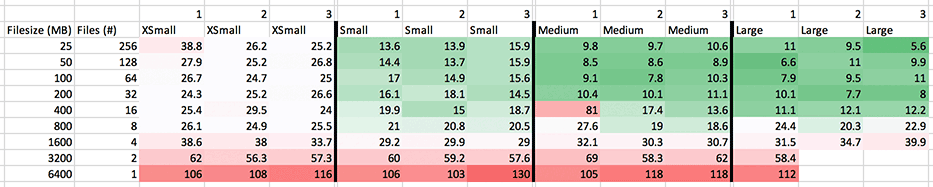
Storage is decoupled with compute in Snowflake so I think it is normal to see a larger variance than a traditional database, comparing some of the test runs horizontally within the same size warehouse. Nonetheless they all seem tolerable, aside from the odd 80 second blip on the MEDIUM sized server. All graphs going forward are simply going to assume best case performance and use the minimum observed time. Using an average and running more than 3 tests would produce a more accurate result, although minimums will suffice for this article.
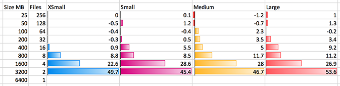
The above is a graph of seconds saved; the bar graphed is the number of seconds saved from the line below it. 6400 MB to 3200 MB – or more accurately, going from a single file to two files, on the XSMALL blue box saved 49.7 seconds. 22.6 seconds is saved going to 4 files or threads; an additional 8.8 seconds at 8 threads. There is a tiny improvement at 16 although that could simply be test variance. We know the unload statement dumps 8 threads at a time per server; it looks like the same is true for the copy statement on ingest. If this is the case, we should expect to see the same diminishing returns on the SMALL 2-node magenta cluster at 16 threads, which we do observe: 5.5 seconds saved going from 8 to 16 threads. This means we want our file count and virtual warehouse size to result in each server node working on 8 files at a time. Continuing to look upwards on the XSMALL blue bars, we can see the negative numbers indicating a longer amount of time was taken; this may just be attributable to test variance/noise, or this may be the result of the additional overhead from more S3 GET operations, which would compound and be most observable on a single node.
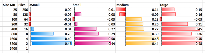
The above is another view of the same data; again read from bottom to top. For XSMALL 1-node in blue we see 3200×2 is 0.47x the time of 6400×1. The big improvements decline after 800×8. This is clear at 16 for SMALL – less clear on the others, although given enough tests I think they would clearly show the diminishing returns at 32 for the MEDIUM (4 nodes * 8 threads) and 64 for the LARGE.
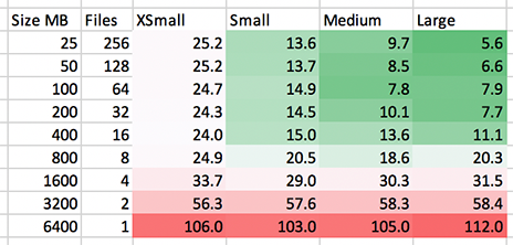
How does load of this particular data set scale out with growing the virtual warehouse? We want to see results become faster and greener as we move from the left to the right. Anything in red is wasted resources to an unsaturated cluster; a very expensive cluster as we move to the right. Not only do we want to see performance improve as we move to the right, but since we’re adding twice the servers, the ideal case is really seeing 2x performance. This is what we see:
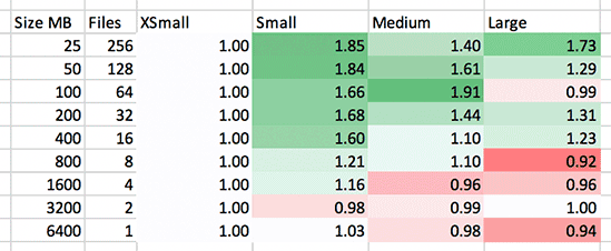
The MEDIUM to LARGE at 100 MB seems to be an odd anomaly. What we’re really looking for here is green, and a strong green at that, to justify spending the additional money on the larger virtual warehouse. Considering the increase in cost, I would hesitate to ramp up to larger clusters for ETL ingest unless they are sure to be saturated and fully utilized. Note these numbers only reflect the L in ETL and not the T – subsequent transforms and movement of the data within the database would likely result in some improvements in these numbers.
Snowflake ETL Design: Presentation Layer Considerations
Very often data is not loaded directly to a presentation layer table that reporting is done off of, but a staging table where data is initially ingested. This data is then carried forward with a process then placed into the final target presentation table for reporting. One example of this is an ELT operation of assigning raw dimension table inputs with a surrogate key on the presentation layer dimension table in a typical warehouse. Another example is fact data loaded to a staging table, which is promoted to the presentation fact after a series of dimension table surrogate key lookups.
Aside from throwing brute force computing and the clever design of Snowflake’s architecture at serving queries, there’s still more that can be done to best take advantage of these features. In particular at this stage, assuming best practices for general data warehouse and table design have been applied, how the table is loaded has a significant effect on performance. This is where the ETL/ELT opportunity lies – in promotion of data from the ingest/staging table into the presentation table. Inserting the data in a sorted order, or defining table cluster keys should be considered in the design for optimal report time queries by users. Micro-partitions are influenced by both of these techniques as noted in the article on Snowflake performance tuning.
Stay connected