

What’s the best way to extract data out of Snowflake? I’m unloading it from Snowflake to S3 and am curious of how to maximize performance. An AWS lambda function I’m working on will pick up the data for additional processing.
Single File Extract
The test data I’m using is the titanic data set from Kaggle. This initial set has been rolled over to represent 28 million passenger records, which compresses well on Snowflake to only 223.2 MB, however dumping it to S3 takes up 2.3 GB.
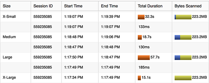
Running far too many tests than I should for this – how do we fare with extracting to a single file? It is interesting to note the surprising amount of variance given that I am the lone user on the system. These dumps aren’t just 1 or 2 seconds different but range from 49 to 78 seconds – a huge range. This cannot be explained by any local caching of data that may have occurred as I resized warehouses and possibly got nodes within the same cluster pool; because 223 MB is simply too little and too fast to read to explain this disparity in time.

What should be the biggest takeaway here is also that the times don’t change – this is because we are not benefiting from a larger virtual warehouse. The number of nodes do not matter because Snowflake doesn’t route all it’s i/o through a master head node but through the nodes that make up the Snowflake architecture. Regardless of the virtual warehouse size, only 1 server node within it is being used to write a file when we are asking for a single file output; we have forced the degrees of parallelism to 1.
This is, of course, not an ideal state for maximizing performance. Keep in mind that this export is only suitable for small datasets, and was achieved by setting single=false in the copy statement. What Snowflake really wants is multiple files, we need to shred the data!

Multiple File Extracts
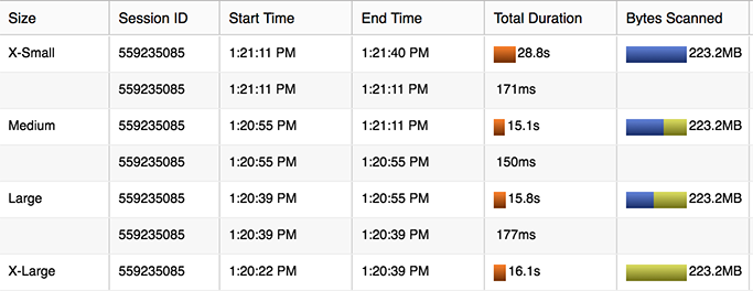
Before we get into the results of this test, note some of the surprising inconsistency observed yet again. The average case over time is certainly going to be better as the virtual warehouse cluster increases in nodes, however at the individual test level the behavior can vary both largely and surprisingly frequently.
Note that we also need enough data flying around to really leverage those additional nodes in the cluster. Based on the file size limit, we’re only going to write x many files, and at some point we simply aren’t asking the nodes to do enough apiece. The nodes are not as saturated as they could be, so in the case below the performance doesn’t actually improve as the cluster grows.
What’s the node behavior actually going on here, how many files is that? Observing the naming convention of the files as we grow the cluster we figure out the meaning behind them. We’re now producing many files after setting the option single=false; also specified is a max_file_size in terms of bytes.
ALTER WAREHOUSE "COMPUTE_WH" SET WAREHOUSE_SIZE = 'XLARGE' AUTO_SUSPEND = 120 AUTO_RESUME = TRUE COMMENT = '';

COPY INTO @S3_SUPPORT/dumptest/xlarge/passengers_28m_parts.csv
from (select * from passengers_28m)
file_format = (format_name='default_csv' compression='none') header=true overwrite=true single=false max_file_size=200000000;
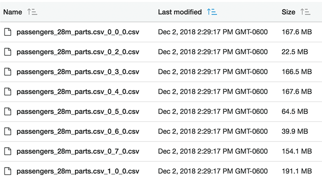
Here we can see that the filename is appended with a suffix for each shredded data thread being extracted. 0_0_0.csv, 0_1_0.csv, and so on. There are 8 threads being extracted per node; so a 4-node medium sized cluster will be simultaneously writing 32 files. In terms of the naming convention of x_y_z, here’s what the numbers appear to indicate:
- x = the server number, starting with 0
- y = the thread, 0-7
- z = the round of threads, starting at 0
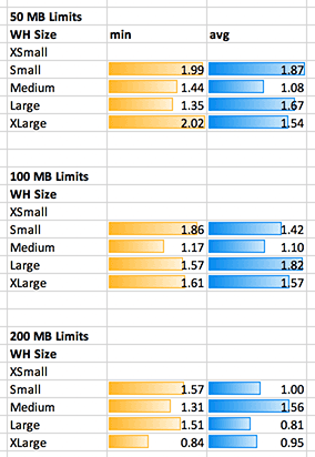
I ramped this up to an even larger table; 140 million records; 1.1 GB compressed on Snowflake. This is over 11 GB of csv data when dumped to S3. I ran three tests using various file size limits. My own lambda function can only work with 50 MB files so it’s the limit I will use in production for my own use case.
- Multi-file write with a 50 MB limit
- Multi-file write with a 100 MB limit
- Multi-file write with a 200 MB limit

We observe the following:
- There’s a surprising amount of variation from test to test, which we can see in the standard deviation as well as visually on the 4 test iterations.
- The max time was surprisingly worse on some larger clusters, and perhaps even more surprising is how large a gap there is between max and min times.
- Average times mostly improved – up until the point where the number of files produced divided by the number of threads was less than two.
- One of the largest improvements was made by moving from 50 MB to 200 MB files. However… there’s not a great obvious reason for this; it doesn’t take that much time to close or open a new file. Although we are not exactly writing files here, but writing objects to S3 – nonetheless this seems like a surprising amount of overhead.
Can we figure out anything from the naming and write dates of the files? Let’s take a look.
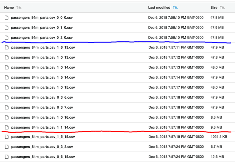
Check out thread 3 on server 0; 0_3_z. The colored lines represent where I’ve skipped over files. Thread 3 rounds 6, 7, and 8 (z) complete along with rounds 13, 14, and 15 of other threads. 0_3_8 is only 6.7 MB – it’s a final write. Thread 0_3 completed rounds 0-9; looking over the other files, thread 0_2 completed rounds 0-17.
So, it looks like thread 0_3 really lagged behind the others. The data is the exact same data rolled over many times in the table; there’s no reason for any thread to lag this far behind any others. Yet, for some reason it seems to have; this type of situation happening multiple times is probably the explanation as to why run times can change so drastically from one test to the next. This certainly seems the best explanation we have available for this observance, although it seems to be quite random when it occurs. The more files produced, the less likely it seems we’ll experience it.
Time Efficiency
We want to keep virtual node write threads saturated, and each atomic S3 object PUT request appears to be what is robbing us of time as we write smaller files/objects. To minimize the number of these commands, if an option we simply can write larger objects. Ie, use 200 MB extracts rather than 50 MB extracts if it makes sense for your data, or larger of course. To achieve the best average case performance for extract time, it looks like the largest cluster should be chosen where (# files / (# nodes * 8)) is greater than 2. This seems to safely make sure we 1. efficiently saturate nodes with write threads and 2. minimize the effect of laggard threads over time and iterations.
Cost Efficiency
Snowflake warehouse costs are charged in credits per hour, with credits going towards the number of nodes. Assuming a virtual warehouse turned on/off for only the duration of a query, anything that scales linearly will cost the same amount. Ie. 4 nodes * 15 seconds is the same cost as 1 node * 60 seconds. Under the same cost and linearly scaled performance, one can simply choose the warehouse size that gets the operation done the fastest. How does our extract scale in this case? If linearly (or better) we would expect to see a 2x jump going up from one virtual warehouse size to the next. However, this isn’t actually what we observe in our test case.
Although we are definitely getting the job done more quickly as we scale up the cluster, our costs are not scaling linearly with the number of nodes in the virtual warehouse; our costs are rising as well. In the 50 MB case, the XLARGE is 16x the nodes and 16x the cost of the 1 node XSMALL – however the average time was only a 5.23x improvement; the best time a 7.77x.
Conclusion
Multiple factors may go in to how you are sizing and running your extracts; for example, my next process has a limit on receiving 50 MB chunks, so it is going to dictate that I must write many smaller files. You may only care about speed in your process, or cost and speed may both be factors. The test case shown here was with this specific set of data – due to compression of your data and/or complexity of query, other factors may influence your own extracts. I hope this article helps as you consider the factors and balance out your own performance and cost needs in configuring your extracts. I am also quite curious in regards to the varying performance and laggard write threads observed here and if anyone can provide additional information on what’s going on there.
Viewing the files for a 48 file dump on a large system; rather than the expected [0-7]_[0-7]_0, the files were [0-6]_[0-3]_[0-3]. This is pretty surprising given that one node appeared to do nothing. Why would the others go more rounds rather than have less but more parallel rounds? I don’t know why we don’t see a single round of everything written at once, although this behavior would explain why we also don’t always see the gains we might expect when upsizing the warehouse.
UPDATE:
After several frustrating hours, I found the limit statement was creating a lot of problems from me in a recent project. It appeared to do two things, both pretty problematic for an extract:
- Collect all data onto a single node, node 0 in my cluster’s case.
- Write the data out in a single thread!
My 48 files ranged from 0_0_0 to 0_0_47. The naming convention implies they were made serially in 48 rounds – as did the total time they took and individual file timestamps as well. Avoid the limit!
Stay connected