

Snowflake Clustering Keys seem to have been a more recently introduced, but extremely powerful, feature of the Snowflake database. They’re a simple feature with a large impact on query tuning and run-time query performance, particularly during scans. There’s a clever concept in Netezza called zone maps, where info about each row is written into the extent/page on disk of what data is contained in it, for integers and dates. During the table scan, this metadata of information is read about the block to decide whether to go through the actual effort of using i/o resources to retrieve the block. Ordering the data based on frequently restricted fields yields large improvements in reducing scan times. Oracle also introduced these in 2014 I believe, however it is 2018 and my bet is the odds an Oracle DBA does anything with them or even knows anything about them is like 1 in 5, because Oracle is the opposite of simplicity that these other platforms are delivering like Netezza and Snowflake.
Snowflake is a columnar compressed database. It is doing something similar with the way it stores data in micro-partitions, which are 50 to 500 MB chunks of (pre-compressed) data. It doesn’t appear we have control over compression, which is fine; they are probably picking the optimal ones, plus having to manually do it has now been removed as a step for DBAs or developers to ignore.
The below image taken from their documentation shows the impact of how the data is laid out on a table during query run time. The query here is being restricted on the value ‘R’, and what we’re looking at is how many micro-partitions we need to actually read to satisfy this query. While Netezza was limited to date/int values, Snowflake is not – I believe the way a columnar compressed database works, it’s simply storing an integer representing the value R… so it’s easy to keep track of this (always int) metadata to decide whether to read a partition or not. That’s what I’m going to roll with conceptually in any case. The 0 to 100 clustering ratio is something Snowflake calculates to try and advise how well the table is set up for querying quickly and making optimal use of i/o resources.
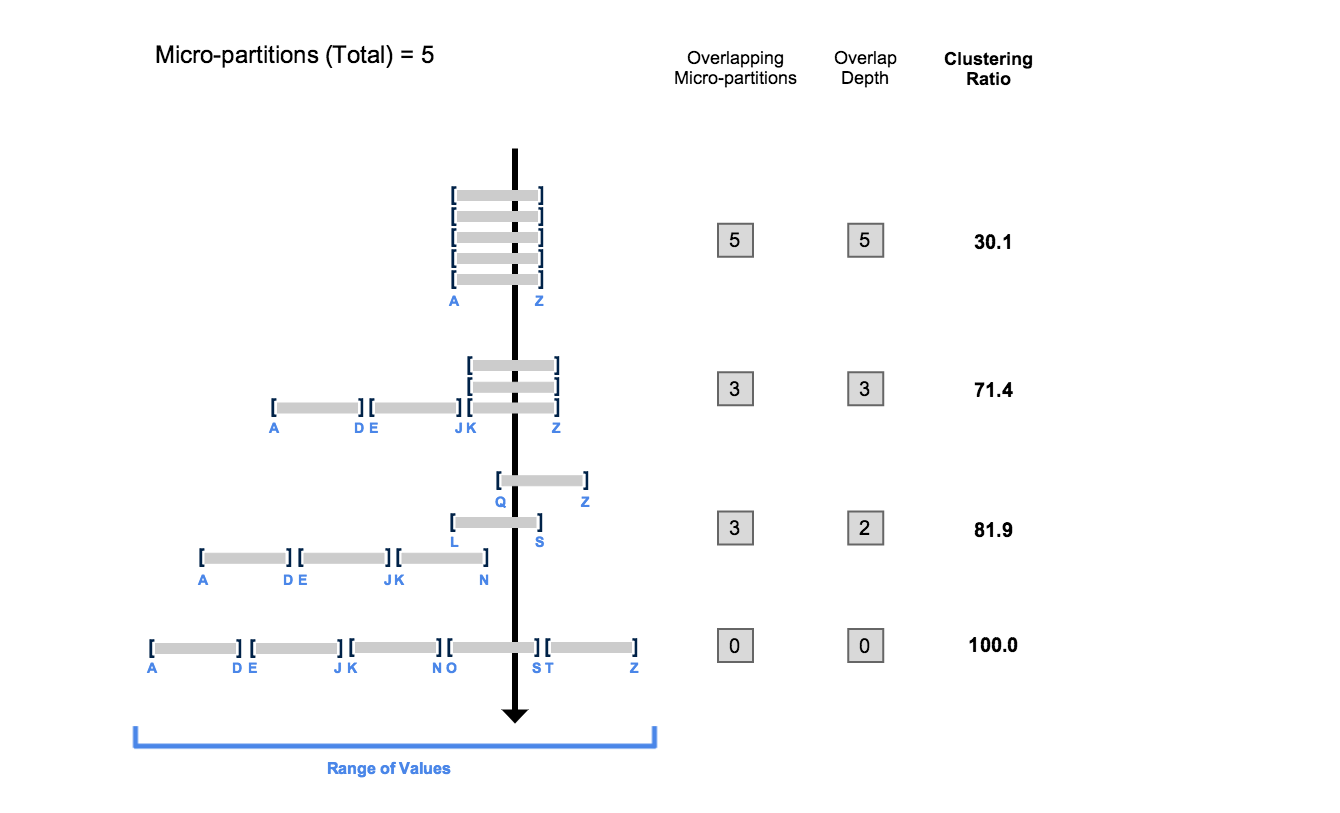
At the top we have the worst case scenario; bulk data in willy-nilly (technical term) order, in which case we need to read every partition. Let’s pretend that’s 50 MB; we need to read 250 MB to find the R records. There may not be any in the first partition, but it does contain both Alpha and Zulu so we need to read it anyway. As clustering improves down the table in different ways the data could reside in it, we see our scan going from 250, to 150, to 100, to just 50 MB of data being necessary to read. Needing to only read 20% of the table now is going to give us a serious boost in performance.
Next we have a pic on what the data looks like as originally ordered, then a set of clustering keys is applied to this table. The data is mostly already ordered on date; perhaps to imply something like incremental ETL batches. However we can see that filtering on id = 2, we’d have to read all 4 partitions. A recluster command based on using date and id yields the second set of more orderly clusters.

Note the data is perfectly in order in the reclustered set, however the the id is not. Why is this? My guess is it is to indicate that clustering means that are choosing the most effective way to cluster the data internally – somehow – and trying to show that they don’t simply mean sorting the data in order of cluster key precedence. Netezza has a similar feature; rather than manual sorts being performed, a table can be cluster based; the data is originally insert in whatever order is set by the ETL, however a call to refresh after that uses an algorithm to try and cluster alike keys together on disk. Generally speaking, on that system, a sort seems to work best when always restricting on column x (date) and sometimes the second sorted column y (product id) – whereas a CBT may work best on a table with fields of similar cardinality and competing rather than complimentary where clauses, such as sometimes being restricted on column a (product type) and sometimes column b (product package type) or sometimes both. We’ll try to see how similar this is to Snowflake cluster keys, which seem more alike Redshift (Amazon AWS columnar db) keys, which are specifically noted as sort keys.
To see how big a difference these make, using the small compute and a large table is the way to go. I wanted my own copies as I don’t know how Snowflake set theirs up (probably clustered on date at least) – I started copying the 1.3 TB TPCDS_SF10TCL schema STORE_SALES table… still on the small size node.

Eventually I figured out this was a HORRIFIC MISTAKE. Hours later I canceled this, nicely enough you can see how much progress it actually made. This was pretty unbearable, I can see why the size is ramped up when you want to load something serious. This is a CPU intensive load; reading all the data involved decompressing it, stitching rows back together, ordering them, then compressing it on write.


Life got a lot better stepping up my game to the big daddy 2X-Large nodes, although that went from 2 credits an hour to 32 credits an hour, so I certainly started blowing through my new account granted $400 allocation a lot more quickly. I also switched to the slightly smaller store_returns table.
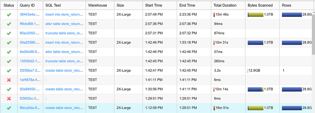
From the bottom up you can see me creating a store_returns ordered by date, item; one ordered by item, date; then one I created with a limit 1 statement (it didn’t like create table as with a limit 0), a truncate, then an insert ordered by item and date. Which oops, I did twice. What is interesting to see is the blue/green; hovering over each, the green said remote, and the blue said local. Per the doc, the green is read from s3 storage, while local is read from local SSD drives on our warehouse nodes. SSD data cache? That is a totally awesome feature! I wonder if the size of the cache grows based on your node, or just based on what you are hitting, given the architecture is supposed to treat compute and disk separately and elastically address bottlenecks in either.
We need to write the same amount in all cases here. As I recall running these, the query was still running for some time after the read was completed; the compress and write through to disk takes some time. We can see the SSD caching itself was responsible for a good 6 minutes of saved read time. I do have a question though – why is my 2:07 repeat of my 1:42 workload coming from remote disk instead of cached SSD? As an aside you may notice I wasted 15 minutes of idle time on this expensive box between these – don’t do that! I’m the only one on my warehouse, and I haven’t done any activity between these. So why did my data cache not persist? I assume it expires shortly, or perhaps it is some shared layer quantity of storage with other Snowflake customer allocations?
Scan Test
I’m using the store_returns table from the TPCDS set, which depending on how I’ve sorted or clustered it, lands around 15.5 MB per micro-partition. I’ll also note the data is pretty artificial and synthetic vs. any real fact tables I think anyone works on, given how it’s all numbers and how everything seems to be fairly evenly spaced out, ie. every store has a similar gazillion amount of sales, as does every product, etc etc. I’m just going to filter on a month and some stores and see how long it takes to get my answer. I’ve also filtered on just the date, and just the store, to compare those results.
select avg(sr_net_loss)
from STORE_RETURNS_CL_DATE_STORE
where sr_returned_date_sk between 2451636 and 2451665
and sr_store_sk in (1646, 1168, 1669, 1742, 1792, 1334, 542, 613, 1400, 314, 1723, 1729, 109, 679, 104);
The full query will need to pull off 3 columns to do it’s work, and we should see micro-partitions eliminate a full table scan as they decide to only read those partitions where the data might reside. How well do different techniques work? I was surprised to see what I thought would work well – and probably would have worked better on Netezza, didn’t really work out the best here. It was also interesting to see the change in cluster results.
Snowflake provides a really nice query profiler which is where I’m pulling these numbers from; the less partitions we read/less time we spend scanning the better.

The results – of data ordered by store+date, date+store, then clustered by date+store, store+date:
I’ll note the partitions scanned data bars are relative to eachother among the whole set, but the MB scanned bars only relative to eachother within the query. The three respective results are a filter on store only, dates only, then the combination of date and store as in the sql above.
- I actually expected ordered by date, store to possibly win – yet ultimately it lost vs. these other methods.
- I did this thinking of data in the row-store world, on Netezza 3MB or even 128k level zone maps, where they would have been very complimentary sorts. However at 15 MB and in the columnar world, it seems arguable that one should go straight off for clustering by the highest cardinality common filter (??)
- Alternatively this may be the result of the very synthetic data and this query, definitely worth exploring with your own tests done with real data and real queries.
- The quickest pruning was for single field filters (only store or only date) was done on data sets ordered by that field. This falls in line with expectations.
- Clustering is not just a sort – although I suspected it might be, that does not appear to be the case; it is employing some kind of algorithm.
- Clustering order matters! – this was another expectation broken – I figured whatever fields were being clustered on could be input in any order – if the data was placed by an algorithm instead of simply sorting – and result in data being laid down across the system in the same way. However this is not the case.
- I’m unclear on the relationship of micro-partitions to bytes scanned; although all my tables have a size/# of partitions = about 15 MB, that relationship isn’t the case above. For example, looking at the first table and dividing MB by micro-partitions, we get more like 1.1 MB. Table 2 (ordered by date, store) scanned 22,978 of 60,924 partitions; ~38% of them, yet bytes scanned was 27.1 GB – meanwhile the entire table is 945.5 GB. How to reconcile or interpret these numbers? I’m unclear. What I’m really looking for is reading the least micro-partitions either way though.
What is also interesting is that Snowflake has a trio of functions for exploring cluster data – one need not even run the query to see how many partitions will be read! This can be done on a per column or set of columns basis, and can be done with the actual restrict in a where clause as well. These appear to be free queries as well that simply read metadata; my warehouse is currently suspended yet these queries are working for me.
It seems the most useful one to me is leveraging SYSTEM$CLUSTERING_INFORMATION and applying a real restrict to see the amount of micro-partitions read.
select
SYSTEM$CLUSTERING_DEPTH('STORE_RETURNS_ORD_DATE_STORE', '(SR_store_SK, sr_returned_date_sk)', 'sr_store_sk in (1646, 1168, 1669, 1742, 1792, 1334, 542, 613, 1400, 314, 1723, 1729, 109, 679, 104) and sr_returned_date_sk between 2451636 and 2451665'),
SYSTEM$CLUSTERING_RATIO('STORE_RETURNS_ORD_DATE_STORE', '(SR_store_SK, sr_returned_date_sk)', 'sr_store_sk in (1646, 1168, 1669, 1742, 1792, 1334, 542, 613, 1400, 314, 1723, 1729, 109, 679, 104) and sr_returned_date_sk between 2451636 and 2451665'),
SYSTEM$CLUSTERING_INFORMATION('STORE_RETURNS_ORD_DATE_STORE', '(SR_store_SK, sr_returned_date_sk)', 'sr_store_sk in (1646, 1168, 1669, 1742, 1792, 1334, 542, 613, 1400, 314, 1723, 1729, 109, 679, 104) and sr_returned_date_sk between 2451636 and 2451665');
Order matters in the second parameter as well. Given that is the case I don’t feel like it’s super reliable when passed multiple columns without additional actual restricts on the data. While these are straightforward to use for tables you’re clustering or ordering by a single field (in which case it appears you’d be best off ordering potentially anyway) for multiple fields they are a little trickier to interpret. I’d go with ideally passing in real predicates and looking for queries with the smallest total count from CLUSTERING_INFORMATION. If just using fields, I would consider looking for a higher constant count from the same function, which is a field that also appears order agnostic about the clustering keys passed in. This particular histogram (also from a different query) is showing that for 58,901 values, only 1 micro partition need be searched (very good!) but for 866 values, 512 would need to be searched to see if the data really existed there or not (not so great!) – the general goal would be to have the brunt of the data skewed toward the top/lower end of the histogram.
My takeaways from this;
- It’s probably best to insert your ETL data in some type of order – if nothing more than to have some optimal scan speed benefit until you take the opportunity to cluster it. Perhaps the recluster is even a best practice to apply post-ETL, depending on how heavy the operation is (??) Per the reclustering documentation, clusters can reach a constant state where a cluster cannot be improved and will thus not be touched – so it would be nice if this became a light operation that only did work on your recently introduced data. If it’s not that light perhaps it can be relegated from post-ETL to a weekend activity.
- At least for this set, the complimentary (in my mind) sort of date then store was sub-optimal; perhaps the best fact clusters are done listing the highest cardinality (and still frequently used) filter condition first. Followed by the usually present date or time dimension.
- One should likely order or cluster the data as part of ETL, and absolutely do so for any initial/historical data load.
- This seems to be the one and only knob to turn in Snowflake, and it’s worth investing the time to understand and use it.
- It would be a super nice enhancement if snowflake logged query history metadata in a more accessible way for you, so that you could see something like the number of times a table is accessed, and which columns are used in joins, and which columns were used in restricts.
Additional Clustering Considerations from Snowflake
- Per the doc, a clustering key is not necessary for most tables, and in many cases data will benefit from this technology anyway, particularly for tables with dates/timestamps. However the reality is, if you want to optimize performance, you’ll have a clustering key or a load approach designed to get the most out of these. The fact will indeed come in naturally in order more or less from the time dimension, but you may want some other element in there too – and the historical loads cannot be trusted to be in a time dimension order unless you make them that way.
- Per the doc, Snowflake automatically sorts data as it is inserted/loaded into a table – although Snowflake doesn’t actually know what you’re restricting on. I would read this as within a 50 to 500 MB buffer of data, pre-compression, Snowflake sorts within it to create the 15 MB micro partition.
- A recluster of a table with clustering keys is a lighter operation than a recreate of the table with a sort – because a clustered table has the ability to create-static partitions (likely meaning 100% the same values for the cluster key(s)) which will not benefit from any move. The ctas alternatively would always be a full table operation.
- Snowflake’s documentation tip recommends clustering keys set on a table to go from lowest to highest cardinality; note this is what I tried with date, store. (Date actually is technically higher cardinality, although not within the limited scope of my 30 day query or a normal day’s worth of data, ie. 1 day will have data from 1900 stores.) As always – best to do your own test on your own data and see what you discover!
- Also of note and interest is that a cluster key can be an expression – the tips not an example of timestamp on a fact table and how being very high cardinality could produce additional overhead; I believe what they are referring to would be reclustering acting like full table scans in this case. What they advise makes a lot of sense: to set the clsuter key on to_date(timestamp).
- Snowflake recommends that reclustering be done on a separate appropriately sized warehouse – ie. do it in something like the ETL warehouse – not your users querying the database warehouse – and right-size it for the operation and table size at hand.
- Storage costs of a reclustering can be a factor if a significant amount of rows are moved, as old copies of the table are stored for time travel and fail-safe features.
- Partial reclusters are supported – pretty neat actually. One can specify up to a certain size as well as withing certain parameters, ie. up to 2 GB of data, but only that with a load_dt since last Sunday.
alter table t recluster max_size=2000000000 where load_dt >= '4-Mar-2018';
I tried playing around with joins also to see what the effects were on Snowflake clustering join keys as well.
Stay connected